If you have not yet read the last post Stream Ciphers, Random Numbers, and the One-Time Pad it is highly recommended you go ahead and read that to understand the stream cipher.
Goal: Construct a stream cipher that is small in hardware.
This post makes the most sense when thinking about the hardware like most cryptosystems. I am a Mathematician and Computer Scientist, so hardware is not my specialty. For those who have learned computer architecture, some of these things should look familiar to you.
Shift Register Stream Cipher
As we learned in the last post, stream ciphers use a stream of bits that are generated by a random number generator(RNG). We discussed those types of RNGs and talked briefly about the one we need the Cryptographically secure Pseudo Random Number Generator(CPRNG). One of the ways we are going to create a CPRNG is by using linear feedback shift registers(LFSRs). LFSRs are implemented in hardware using flip-flops. We will introduce a basic 1LFSR which in practice is quite weak. However, we will show a way to make it stronger such as in the A5/1.
Do be aware though that today stream ciphers that use LFSRs like A5/1 are not considered secure, and should not be used in practice. That does not mean all stream ciphers are weak, for example ChaCha20 and AES-GCB. I state this to show why it is important to learn about stream ciphers, and learning with easier methods like with LFSRs will give you a good foundation for the future.
Linear Feedback Shift Registers (LFSR)
An LFSR is built with a stream of clocked flip-flops making a feedback path. The number of these flip-flops gives us the degree of the LFSR. Meaning if we have n flip-flops, the LFSR is said to be degree n.
Here is a model of a flip-flop, and beside it is a computer architecture model for the clock, input and output:
Example
Let’s consider a simple LFSR of degree n = 3, recall that means the LFSR has 3 flips-flops FF2, FF1, FF0, and the internal bits inside each flip-flop will be denoted by si and are shifted to the right with each clock tick. The rightmost bit will be the output, and the leftmost bit is computed in the feedback path with an XOR sum of some of the flip-flops. Since XOR is a linear operation this circuit is called linear feedback shift registers. For this example we need to assume an initial state of (s2 = 1, s1 = 0, s0 = 0), thus here is the example below:
Notice that the pattern starts to repeat at clock cycle 6. Thus, this LFSR has a period length of 7, and the output will look like:
0010111 0010111 0010111 …
Mathematical Description
You may be able to notice after reading my past blog posts that this can be represented very simply with a formula that determines the output of our LFSR. Let’s look at how we could compute si from our example, assuming we have the initial state bits.
s3 ≡ s1 + s0 mod 2
s4 ≡ s2 + s1 mod 2
s5 ≡ s3 + s2 mod 2
…
si + 3 ≡ si + 1 + si mod 2
where i = 0, 1, 2, …
This was a simple example, but hopefully, you have a better grasp of what a LFSR is. Next, we will look at constructing a general LFSR so we can make the period length longer.
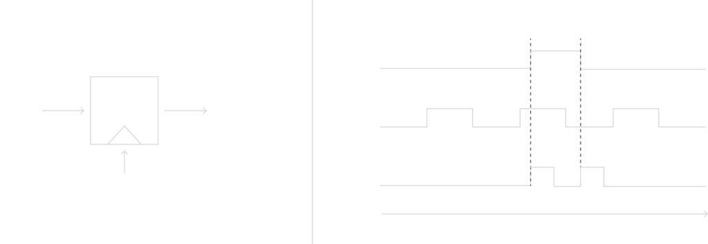
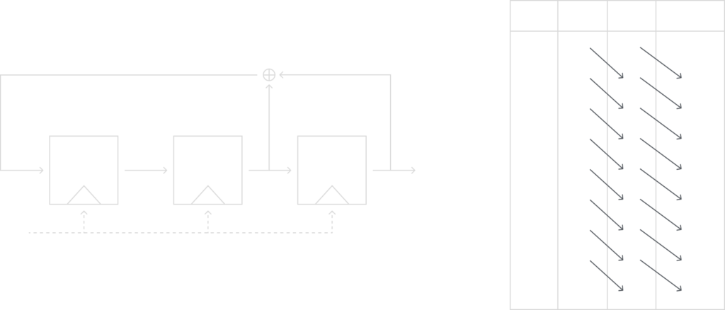
General LFSRs
The general form of an LFSR of degree n is shown in the model below. It shows an LFSR with n flip-flips and n possible feedback locations when all combined by the XOR operation to replace the leftmost bit.
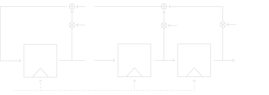
I will introduce the new notation to determine if a feedback path is active or not(ie if that will be included in the XOR or not) is determined by the feedback coefficient p0, p1, …, pn – 1:
- If pi = 1 (closed switch), the feedback is active.
- If pi = 0 (open switch), the flip-flop output is not used in the feedback path.
Therefore, it is now easy to write a mathematical description for the feedback path. If we just multiply the output of the flip-flop by its feedback coefficient and recall the XOR table. If the feedback coefficient is 0, the bit is unchanged and if it is 1 then it is flipped. The feedback coefficients are crucial to the output sequence produced by the LFSR.
Just like in our example of the degree n = 3 LFSR, we can write a general mathematical description for our general LFSR with the corresponding feedback coefficients:
sn ≡ sn – 1 pn – 1 + … + s1 p1 + s0 p0 mod 2
sn + 1 ≡ sn pn + … + s2 p1 + s1 p0 mod 2
In general:
s i + n ≡ ∑j = 0n – 1 pj si + j mod 2
Where, pi ,si ∈ {0, 1} and i = 0, 1, 2, …
Due to the finite number of states, the flip-flops can be in, all LFSRs repeat periodically, just like in the example above. Additionally, an LFSR can have different period lengths depending on the feedback coefficients. The theorem below gives the maximum length of an LFSR period given its degree:
Theorem: The maximum sequence length generated by an LFSR of degree n is 2n – 1.
To explain why the theorem is true, consider how the possible combinations of the flip-flips can be either 1 or 0. The possible combination is 2n but it is impossible for all the flip-flips to be 0, so you subtract 1.
Note that only certain configurations of the feedback coefficients give a maximum-length LFSR.
Examples
1) Consider an LFSR of degree n = 4 and the feedback path (p3 = 0, p2 = 0, p1 = 1, p0 = 1), the output sequence of the LFSR has a period of 2n – 1 = 15, this it is a maximum-length LFSR.
2) Consider an LFSR of degree n = 4 and the feedback path (p3 = 1, p2 = 1, p1 = 1, p0 = 1), the output sequence of the LFSR has a period of 5, therefore even though we have more XOR operations the period length is shorter.
Notation
I won’t go into the mathematical background of LFSRs, but hopefully, this was a good introduction to them. But it will be good to know the usual notation of LFSRs so that if you see them you will understand what they mean.
An LFSR is usually specified by polynomials with the following notation: An LFSR with a feedback coefficient vector (pm – 1, …, p1, p0) represented by the polynomial
P(x) = xm + pm – 1 xm – 1 + … + p1 x + p0
For instance, the example given above with feedback coefficients (p3 = 0, p2 = 0, p1 = 1, p0 = 1) can be specified by the polynomial x4 + x + 1. This notation could seem weird, but it has some interesting advantages. One is a way to easily tell if an LFSR is maximum-length by testing if the polynomial associated with it is a primitive polynomial. Which is a polynomial that only has factors of itself and 1. It is pretty easy to test if a polynomial is a primitive polynomial, so it is a good way to test if an LFSR has maximum-length.
Code Implementation
The code implementation of a shift register stream cipher is not too complex. But as I mentioned before, this really makes more sense in hardware but I still try to give a program implementation to these ciphers.
Notice I am not actually using the mathematical equations I introduced but instead am using the shift property to simulate the LFSR. Both implementations would work, and the math-based one would probably be faster. But for the purpose to keep the code short and simple, I choose this implementation method.
					#include <iostream>
#include <string>
#include <bits/stdc++.h>

using namespace std;

void encrypt(string plaintext);

string TextToBinaryString(string s);

int main()
{
    // enter plaintext
    string plaintext = "thequickbrownfoxjumpsoverthelazydog";
    plaintext = TextToBinaryString(plaintext);

    // encrypt function
    encrypt(plaintext);

}

void encrypt(string plaintext)
{

    string ciphertext = "";
    // this is out "LFSR" with degree n = 5
    bool flipFlops[5] = { 1, 0, 0, 0, 0 };

    // iterate over full plaintext message
    for (int j = 0; j < plaintext.length(); j++)
    {
        // get our last bit to be used in encryption
        bool s = flipFlops[4];

        // use the shift property of the LFSR to simulate the hardware verion
        for (int i = 0; i < 4; i++)
        {

            bool temp = flipFlops[i];
            flipFlops[i] = flipFlops[4];
            flipFlops[4] = temp;

        }

        // compute the leftmost bit using XOR based on polynomial x^5 + x^3 + 1
        flipFlops[0] = flipFlops[0] ^ flipFlops[3];
        // encrypt bit
        ciphertext += char((int(plaintext[j]) - 48) ^ s) + 48;
    }
    cout << "ciphertext : " << ciphertext << endl;
}

// this is a function to convert a string to binary
string TextToBinaryString(string s)
{
    string binaryString = "";
    for (char& _char : s) {
        binaryString += bitset<8>(_char).to_string();
    }
    return binaryString;
}
Attack Against Single LFSRs
I alluded at the beginning of this post that a single LFSR is weak in practice, and I will show you an elegant attack against it.
But before you think you wasted your time learning this, we can make it secure by doing what modern-day stream ciphers use. Instead of using a single LFSR, modern systems use 3 LFSRs that feed into each other. This makes it a lot more secure, if you want to know why I will go into depth why 3 is important in my DES post, so make sure to look out for that.
Assumptions
This kind of attack is called a known-plaintext attack, and it is necessary to note some assumptions about the things that the attacker(Malcolm) knows:
- They know all the ciphertext bits.
- They know the degree of the LFSR.
- They know some of the plaintext bits given x0, x1, …, x2m – 1.
Note it is not unreasonable to assume Malcolm has some of the plaintext bits because most files shared have an unencrypted header.
Step 1
Given the assumptions Malcolm can reconstruct the first 2m key stream bits using the mathematical equation we defined before:
si ≡ xi + yi mod 2, where i = 0, 1, …, 2m – 1.
Step 2
The goal now is to recover the remaining keystream bits, and to do this we will need to compute what the n feedback coefficients are.
Recall the general LFSR equation we found earlier:
s i + n ≡ ∑j = 0n – 1 pj si + j mod 2, where, pi ,si ∈ {0, 1} and i = 0, 1, 2, …
Note that we get a different equation for each i, and the equations are linearly independent, with this Malcolm can generate n equations:
i = 0, sn ≡ sn – 1 pn – 1 + … + s1 p1 + s0 p0 mod 2
i = 1, sn + 1 ≡ sn pn – 1 + … + s2 p1 + s1 p0 mod 2
…
i = m – 1, s2n – 1 ≡ s2n – 2 pn – 1 + … + sm p1 + sm – 1 p0 mod 2
Malcolm now has n equations and n unknowns, ie he has a system of linear equations. This now means Malcolm can easily solve for the n unknowns using methods like the matrix method or whatever they like really. Now Malcolm has the feedback coefficients and can reconstruct the entire LFSR and could decrypt the entire message.
Therefore, if an attacker knows at least 2n output values of a LFSR, they can recover the entire LFSR.
Conclusion
We discussed the very important stream cipher. Even though they are less popular than block ciphers which we will discuss in the next post. They have their place in the community like the ChaCha20 and AES-GCB. Even though we discussed stream ciphers using LFSRs like A5/1, today there are many found attacks on them, and should only be considered when using legacy technology that uses them.